

Transformer explanations often begin and end with attention. But attention alone does not explain how a model handles word order, combines information, or generates a response one token at a time.
This article follows the computation from input representations through attention and a complete Transformer block, then compares encoder-only, decoder-only, and encoder–decoder architectures. Along the way, a small numerical example makes the attention calculation reproducible.
In this series, the RAG article concerns the evidence supplied to a model, while the embedding article concerns representations used for retrieval. Here, the focus is what happens inside the model once a sequence is available.
1. Why Move Beyond Recurrent Networks?
Before Transformers, RNNs and their gated variants, including LSTMs and GRUs, were widely used for sequence modeling.
An RNN updates a hidden state as it processes each position:
The dependence on the previous state creates two practical difficulties.
First, positions within a sequence cannot all be processed independently. Computing the state at position three requires the state at position two. Batching helps, but it does not remove that recurrence.
Second, information from an early position must travel through many intermediate states to affect a distant one. Gating helps preserve information, but learning long-range dependencies can still be difficult.
Self-attention provides a more direct path between positions. It improves parallel computation over known sequences and reduces the number of intermediate steps needed for distant positions to interact. That is an architectural advantage, not a guarantee that every long-range relationship will be learned correctly.
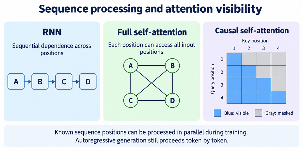
Figure 1. Full attention and causal attention have different visibility rules. The full-attention sketch omits self-loops for clarity; positions can also attend to themselves.
One distinction matters throughout this article: parallel processing during training is not the same as generating every output token simultaneously.
During training, the target sequence is already known, so a causal Transformer can compute predictions at multiple positions in parallel while masking future tokens. During ordinary autoregressive inference, each newly generated token becomes part of the input for the next step.
2. What Does Self-Attention Actually Do?
Consider this sentence:
Emma skipped the trip to London because she had a meeting in Oxford.
A reader normally interprets “she” as referring to Emma. To construct a useful representation at that position, a model can combine information from other positions in the sentence.
This is an illustration of contextual dependence, not a measurement showing that a particular model assigns its highest attention weight to “Emma.” Attention weights vary by model, layer, head, and input. They are also not a complete explanation of why a model produced an answer.
Self-attention computes a weighted mixture of information from the positions that a query is allowed to access.
In full self-attention, those positions may include the entire input sequence. In causal self-attention, a position can access itself and earlier positions, but not future ones.
The result is a contextual representation. For example, the representation of “bank” can differ between “river bank” and “bank account,” even when the tokenizer uses the same token ID for that word.
3. Query, Key, and Value: Three Learned Projections
A library analogy can help introduce the three roles:
- A query expresses what information is being sought.
- A key provides features used for matching.
- A value supplies the information to be combined.
The analogy has limits. Attention does not literally search a library, and its output is not a finished answer. It operates on learned numerical representations.
For an input matrix (X), one standard attention head computes:
If there are (n) positions and the model width is , then:
A common choice of projection shapes is:
Consequently, (Q) and (K) have shape , while (V) has shape. These equations omit projection biases for simplicity.
The weights are learned during training. Separate projections allow matching and information aggregation to use different feature spaces.
At deeper layers, (X) is the representation produced by preceding computation, not the original token embedding table lookup.
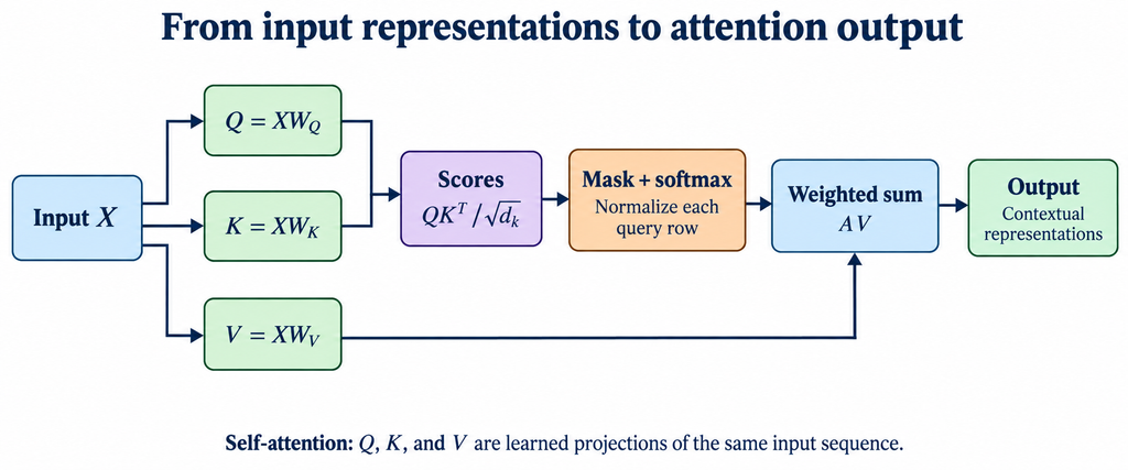
Figure 2. Queries and keys determine attention weights. Values travel along a separate path to the weighted sum.
4. Scaled Dot-Product Attention
For a standard attention head, the computation can be written as:
Here, (M) is an additive mask: allowed positions receive zero, while disallowed positions are conceptually assigned negative infinity before softmax.
Softmax is applied across the key positions separately for each query row. Before any attention dropout, each valid row sums to one.
The computation has three stages:
- Compare queries with keys using dot products.
- Scale the scores, apply the mask, and normalize them.
- Use the resulting weights to combine value vectors.
The output (O) contains one representation per query position. It is an intermediate representation, not a probability distribution over vocabulary tokens.
Why divide by the square root of the key dimension?
Under a simplified assumption that query and key components are independent, have zero mean, and have unit variance, their dot product has variance proportional to .
Dividing by counteracts that growth in scale. Very large score differences can make softmax highly concentrated and produce small gradients through it.
This does not mean that attention should always be uniform. Focused attention can be useful. The scaling controls score magnitude; it does not guarantee good training or a particular attention pattern.
The original Transformer paper introduces this scaling, along with the attention, masking, and block structure discussed here.
5. A Small Attention Calculation You Can Verify
Take one query, three keys, and three value vectors. These are invented teaching values, not activations from a trained model.
Let:
Because , dividing the dot products by gives:
Assume all three keys are visible. Softmax then gives:
Now choose:
The output is:
The following example uses only Python’s standard library:
from math import exp, isclose, log, sqrt

q = [sqrt(2), 0.0]
keys = [[log(2), 0.0], [log(3), 0.0], [log(5), 0.0]]
values = [[1.0, 0.0], [0.0, 2.0], [2.0, 2.0]]

scores = [
    sum(qi * ki for qi, ki in zip(q, key)) / sqrt(len(q))
    for key in keys
]

# Subtracting the maximum improves numerical stability.
offset = max(scores)
exponentials = [exp(score - offset) for score in scores]
weights = [value / sum(exponentials) for value in exponentials]

output = [
    sum(weight * value[j] for weight, value in zip(weights, values))
    for j in range(len(values[0]))
]

assert isclose(sum(weights), 1.0)
assert all(
    isclose(actual, expected)
    for actual, expected in zip(output, [1.2, 1.6])
)

print([round(weight, 4) for weight in weights])
print([round(value, 4) for value in output])
Expected output:
[0.2, 0.3, 0.5]
[1.2, 1.6]
This example separates two ideas that are easy to blur: query-key matching produces the weights, while the values determine what is mixed.
6. Why Use Multiple Attention Heads?
A sentence about an order can contain several interacting details:
Inventory was reserved successfully, but the payment callback failed.
Useful representations may need to preserve entities, actions, statuses, and dependencies. Multi-head attention allows multiple attention computations to operate in parallel using different learned projections:
Their outputs are concatenated and projected:
It is tempting to label one head “syntax” and another “causality,” but those roles are not assigned by the architecture. Heads can learn overlapping patterns, and a single head is not restricted to one semantic relationship.
These equations describe standard multi-head attention. Variants can share key and value projections across query heads, so the arrangement should not be assumed to describe every modern model.
7. How Does the Model Know the Order?
The words in these sentences are identical, but their roles differ:
The customer called the instructor.
The instructor called the customer.
Full self-attention without positional information or position-dependent masks does not itself establish sequence order: permuting the input positions permutes the corresponding output positions.
The original Transformer adds sinusoidal positional encodings to token embeddings. For position (p), its paired dimensions use:
But adding a vector to the input is not the only way to represent position.
Rotary Position Embedding, or RoPE, applies position-dependent rotations to queries and keys. ALiBi introduces distance-related biases into attention scores instead of adding positional embeddings to the input.
These mechanisms affect how position influences attention. None should be interpreted as a blanket guarantee that a model will work reliably at arbitrarily long sequence lengths.
8. A Transformer Block Contains More Than Attention
Attention mixes information across visible positions. The feed-forward network then transforms the representation at each position.
A basic FFN can be expressed as:
It applies the same parameters separately at each position. Unlike attention, this operation does not directly mix information across token positions.
Residual connections and normalization support the composition of these transformations into a deep network.
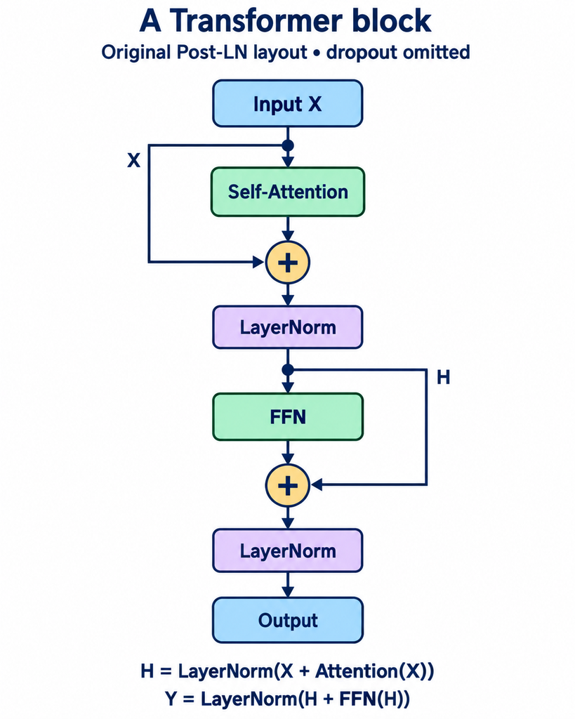
Figure 3. Each residual branch starts at its own sublayer input and ends at the corresponding addition. “Self-Attention” denotes the attention sublayer, typically multi-head.
Ignoring dropout, the illustrated Post-LN block computes:
Notice that the second residual carries (H), not the original (X).
LayerNorm normally normalizes the features within each position’s representation, with learned scale and bias. It should not be pictured as averaging all tokens together.
The figure represents the original Post-LN arrangement. Other architectures place normalization before sublayers or use alternatives such as RMSNorm. The diagram is a foundation for understanding the computation, not an exact blueprint for every current LLM.
9. Encoder-Only, Decoder-Only, and Encoder–Decoder
These architectural families differ mainly in attention visibility and how input and output sequences are connected.
| Architecture | Typical information flow | Example models | Common applications |
|---|---|---|---|
| Encoder-only | Bidirectional attention over the input | BERT | Classification, extraction, representation learning |
| Decoder-only | Causal attention over a growing sequence | GPT-2 | Text and code generation |
| Encoder–decoder | An encoder represents the source; a causal decoder also attends to encoder outputs | T5, BART | Translation, summarization, conditional generation |
These are common applications, not exclusive task boundaries. A model’s training objective and adaptation matter as much as its architectural label.
Encoder-only: represent the input
An encoder can combine information from both sides of a position. That is useful when constructing representations for classification or matching.
However, an encoder does not automatically produce high-quality retrieval embeddings. Pooling, training data, and the retrieval objective still matter, as discussed in the embedding article.
Decoder-only: extend a sequence
A causal language model predicts a continuation using the available prefix.
A typical text-only decoder-only architecture also omits the encoder–decoder cross-attention sublayer. It is therefore misleading to describe it as simply deleting the encoder from the original diagram while keeping the entire original decoder unchanged.
Encoder–decoder: connect two sequences
In the original translation architecture, the encoder processes the source sequence. The decoder uses causal self-attention over the target prefix and cross-attention to the encoder output.
In cross-attention:
- Queries come from the decoder.
- Keys and values come from the encoder output.
The same-input Q/K/V explanation from Section 3 applies to self-attention, not to this cross-attention step.
During training, shifted target tokens are supplied to the decoder with a causal mask. During ordinary generation, the decoder consumes the available prefix and extends it.
10. Why Is Next-Token Prediction So Useful?
An autoregressive language model factorizes a sequence probability as:
A common training objective is the negative log-likelihood:
The next token provides a training target directly from the text. A separate human label is not needed for every position.
Many tasks can be formatted as conditional continuation:
Question: How can I prevent a cache stampede?
Answer:
Translate into English: 我喜欢自然语言处理。
Translation:Complete this Java method:
public User findUserById(Long id) {This provides a common interface for a wide range of tasks. The GPT-2 report explores this relationship between language modeling and multitask behavior.
Still, next-token prediction alone does not guarantee a useful assistant. Data quality, scale, instruction tuning, other post-training methods, and evaluation all affect the result.
Encoder-only and encoder–decoder models remain useful. The choice should follow the task and the available trained models, rather than treating one architectural family as universally superior.
11. What This Means for RAG Applications
In a customer support assistant, retrieval supplies candidate evidence and the language model processes the assembled input.
Consider a user asking about a refund deadline. The retrieved passages include:
- An older policy allowing refunds within seven days.
- A newer policy allowing refunds within fourteen days.
- An unrelated policy for another product.
Attention does not automatically identify the legally or operationally applicable policy. Effective dates, product scope, document authority, and access permissions must be handled by the application and its retrieval design.
A reasonable workflow is to identify the applicable documents, retrieve and rerank relevant passages, then provide selected evidence with clear source labels. The assistant should also have instructions for insufficient or conflicting evidence.
Poor retrieval raises the risk of a wrong answer. It does not force one deterministic behavior: a model might ignore a passage, rely on information in its parameters, report uncertainty, or still produce an unsupported answer.
Likewise, placing a passage inside the supported context window does not guarantee that the model will use it correctly. Too much irrelevant material can increase cost and make the task harder.
For standard dense attention, the number of query-key pairs grows quadratically with sequence length. Efficient implementations can reduce intermediate memory use, but “the model accepts a longer prompt” is still different from “every additional passage helps.”
A small application evaluation can make this concrete: hold the question and applicable policy constant, add irrelevant or conflicting passages, and compare answer correctness and citation support. Such a test measures application behavior; it does not directly reveal the internal meaning of an attention head.
12. What to Take Away
Transformer computation is a sequence of learned operations: position-aware representations, query-key matching, value aggregation, nonlinear transformations, residual paths, and normalization.
That computation explains how information can move through a model. It does not mean that attention weights are a complete explanation of an answer, that every head has a fixed semantic role, or that a model will reliably resolve conflicting evidence.
For an engineer building an AI application, the practical connection is straightforward: better retrieval and better input organization give the model better material to work with. They still need to be paired with explicit constraints and evaluation.
The architecture makes contextual computation possible. The reliability of the finished system depends on much more than the architecture alone.